Beyond the Box Score: Measuring Individual Impact in NCAA Division I Women's Volleyball

The problem: why traditional volleyball statistics don't tell the whole story

Volleyball is inherently a team sport, yet we often evaluate individual players through isolated statistics: hitting percentage, kills, assists, blocks, and digs.

These statistics are useful, but they don't always tell us how much a player contributes to winning.

Consider two outside hitters with identical hitting percentages. One consistently faces strong defensive opponents and receives difficult sets, while the other benefits from excellent passing, favorable matchups, and an experienced setter. Their statistics might look identical, but the circumstances behind those numbers are vastly different.

This raises an important question:

How can we estimate a player's contribution to winning while accounting for the circumstances in which they play?

One possible starting point is plus-minus.

Traditional plus-minus

Plus-minus measures the net points a team scores while a particular player is on the court.

For example, if a team scores 30 points and concedes 20 while a player is playing, that player receives a plus-minus of +10.

This shifts our attention away from isolated actions and toward what ultimately matters: winning points.

However, traditional plus-minus introduces another problem.

Imagine a player on a dominant team. She plays alongside several exceptional teammates, and her team consistently outscores its opponents. Her plus-minus will likely be excellent, but how much of that success can actually be attributed to her?

Conversely, imagine an exceptional player on a struggling team. She might consistently perform well while her team continues to lose points.

Traditional plus-minus cannot reliably distinguish between these situations.

To address this, I explored Regularized Adjusted Plus-Minus (RAPM).

Building an adjusted plus-minus model

Adjusted Plus-Minus (APM) extends traditional plus-minus by estimating the contributions of all players simultaneously.

Instead of assigning every player on the court the same credit for a rally, we construct a linear regression model that considers the players participating on both sides.

The central idea is simple:

A player's estimated impact should depend not only on whether their team wins a rally, but also on who they were playing with and against.

For this project, I worked with approximately 35,000 rallies and 1,131 NCAA Division I women's volleyball players represented in our database.

The regression itself used 21,934 rallies where both teams' lineups and rotations were fully recorded and the score margin within the set was under eight points. I excluded lopsided late-set rallies to reduce the influence of substitution patterns that may not reflect typical competitive lineups.

Constructing the feature matrix

Each rally became a row in a feature matrix, and each player received a column.

The player features were encoded as follows:

+1

Player was on the home team's court.

−1

Player was on the away team's court.

0

Player was not on the court.

The target variable was the result of each rally:

1

Home team won the rally.

0

Away team won the rally.

A simplified feature matrix looks like this:

Rally	Player A	Player B	Player C	Player D	Outcome
1	+1	+1	−1	−1	1
2	+1	0	−1	−1	0
3	0	+1	−1	0	1
4	−1	0	+1	+1	0

With this representation, the model learns a coefficient for each player, estimating their contribution to rally outcomes while accounting for the other players in the model.

The simplified prediction equation is:

Where:

• $\hat{y}_i$ is the predicted outcome of rally $i$.
• $x_{ij}$ represents player $j$'s participation in that rally.
• $\beta_j$ is the learned coefficient for player $j$.
• $\beta_0$ is the intercept.

The full implementation also included serving, rotation, and home-court information.

How does this adjust for opponent difficulty?

An important benefit of this structure is that opponent strength is accounted for implicitly.

Consider a player who consistently competes against strong opponents. Her team may win fewer rallies, but the model simultaneously estimates the contributions of those opposing players.

Because all player coefficients are learned jointly across the dataset, the model can distinguish between outcomes achieved against different combinations of teammates and opponents, provided the data contains enough lineup variation.

This is an improvement over traditional plus-minus, which treats each point won or lost identically regardless of the lineup.

However, this approach introduces an important statistical challenge: multicollinearity.

Why ordinary linear regression isn't enough

In volleyball, players frequently share the court with the same teammates.

Imagine two players who participate in nearly every rally together. If their team consistently wins, how can a regression model determine which player deserves the credit?

The problem is that their feature columns are highly correlated. This is known as multicollinearity.

In ordinary least squares regression, multicollinearity can produce unstable coefficients. Small changes in the training data may cause large changes in individual player estimates, even when the model's overall predictions remain similar.

This is especially problematic when our goal is to produce meaningful player ratings rather than simply predict rally outcomes.

Another challenge is limited playing time.

A player who participates in relatively few rallies might experience unusually favorable or unfavorable results simply due to randomness. Without sufficient evidence, an ordinary regression model can assign an extreme coefficient that does not generalize well.

These challenges motivated my decision to use Ridge regression.

Introducing Ridge regression

Ridge regression retains the same linear structure as ordinary least squares but introduces an additional penalty for large coefficients.

Ordinary least squares minimizes the sum of squared residuals:

Ridge regression adds an L2 regularization penalty:

The loss function now has two components.

Prediction error

The first term measures how accurately the model predicts rally outcomes.

Regularization

The second term penalizes large coefficients by squaring them, summing them, and multiplying the result by $\lambda$.

The parameter $\lambda$, called the regularization strength, controls the tradeoff between fitting the training data and keeping coefficients small.

When $\lambda$ is small, the model has greater flexibility to fit the observed outcomes.

When $\lambda$ is large, large coefficients become increasingly expensive, encouraging the model to shrink them toward zero.

Why Ridge matters for volleyball

Ridge regression is particularly useful for this application for two reasons.

First, it reduces coefficient instability caused by multicollinearity. When two players consistently share the court, Ridge discourages the model from assigning extreme and opposing coefficients without sufficient evidence.

Second, it helps stabilize estimates for players with limited data. Since there is less information supporting their individual effects, the regularization penalty can have a relatively greater influence on their coefficients.

Importantly, Ridge does not explicitly penalize players based on playing time. Instead, the strength of the available evidence determines how much the data can overcome the penalty.

There is also an important limitation:

Choosing lambda with cross-validation

Choosing $\lambda$ is important because excessive regularization can suppress meaningful player differences, while insufficient regularization can produce unstable estimates.

Rather than choosing a value arbitrarily, I used scikit-learn's RidgeCV to select a regularization strength based on cross-validation.

The process evaluates candidate values of $\lambda$, fits models using the corresponding penalties, and compares their performance on held-out validation data.

My initial implementation

I initially searched five candidate values of $\lambda$, which scikit-learn calls alpha: 0.01, 0.1, 1, 10, and 100.

I also standardized the feature columns before fitting the model and included serving, rotation, and home-court indicators alongside the player features.

The implementation followed this structure:

X = np.hstack([context, team_home, player_mat])
y = rallies["home_team_won"]

rapm = Pipeline([
    ("scaler", StandardScaler()),
    ("ridge", RidgeCV(
        alphas=[0.01, 0.1, 1.0, 10.0, 100.0]
    ))
])

rapm.fit(X, y)

Without an explicit cv argument, RidgeCV uses efficient leave-one-out cross-validation by default, with mean squared error as the default scoring criterion.

The selected alpha was 100.

At first, this seemed like a reasonable result. However, two details made me question the implementation.

Problem one: the best alpha was at the boundary

The first issue was that alpha = 100 was the largest value in my search range.

When the optimal value lies at the edge of the tested range, there is a possibility that better values exist beyond that boundary.

By restricting the search to relatively small penalties, I may have prevented the model from selecting the amount of regularization it actually needed.

Problem two: my validation strategy ignored match structure

The second issue was more significant.

Leave-one-out cross-validation holds out one rally at a time. However, rallies from the same match share lineups, opponents, and playing conditions.

As a result, the training data can contain rallies that are extremely similar to the rally being evaluated.

This means that leave-one-out validation may provide an overly optimistic picture of how the model generalizes to completely unseen matches.

Revising the validation strategy

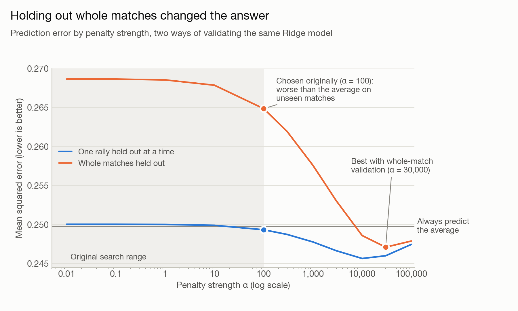
To address both problems, I repeated the search using a substantially wider range of alpha values and five-fold GroupKFold cross-validation, grouping rallies by match.

This ensured that rallies from the same match remained together in either the training or validation fold.

The results changed considerably.

The selected alpha increased from 100 to approximately 30,000.

More importantly, the original model performed worse on unseen matches than a simple baseline that predicted the average rally win rate.

Even after selecting the stronger regularization parameter, the improvement over the baseline was only about 1%.

This was an important finding.

How a model is validated can matter just as much as how the model itself is constructed.

It also reinforced an important distinction: optimizing predictive performance does not automatically produce reliable individual player ratings.

Accounting for serving and rotation

Player participation alone does not capture every relevant factor influencing rally outcomes.

Volleyball is heavily affected by serving and receiving conditions, as well as each team's rotation.

To account for these differences, I included serving information and one-hot-encoded rotation features.

Each team has six possible rotations, producing twelve rotation indicator columns: six for the home team and six for the away team.

One-hot encoding was important because rotations are categorical rather than continuous. Treating rotation numbers as ordinary numerical values would impose an artificial linear relationship between them.

By including these features, the model can account for some systematic differences in rally outcomes associated with serving and rotation, rather than attributing all such variation to individual players.

The fundamental limitation of RAPM

Although RAPM improves upon traditional plus-minus, it still has a fundamental limitation.

It observes who was on the court and whether a rally was won or lost. It does not directly observe how each player contributed to that outcome.

Consider an exceptional passer on a struggling team.

She might consistently deliver high-quality passes, creating favorable attacking opportunities. However, if her teammates fail to convert those opportunities into points, the RAPM model may struggle to recognize the value of her contributions.

Likewise, a player who rarely touches the ball could benefit from consistently playing alongside stronger teammates.

RAPM attempts to separate those effects through lineup variation, but it cannot always do so reliably.

This motivated the second component of my approach: a touch-level win-probability model.

Building the touch-level model

Rather than evaluating players solely through the outcomes of rallies in which they participated, the second model focuses on the actions players actually perform.

Volleyball provides detailed touch-level information, including serves, passes, sets, attacks, and digs.

These actions can be graded according to their quality, providing additional information about individual performance.

I used this information to build a model that predicts rally outcomes based on touch-level events and match context.

Feature engineering and model selection

Each touch grade was converted into a numerical value, ranging from 4 for a perfect touch to −1 for an error.

I then trained an XGBoost classifier to predict whether the home team would win each rally.

The model used 23 features, including:

• Score and set situation.
• Serving information.
• Recent momentum.
• Average grades of serves, passes, and other touches within the rally.

To evaluate performance, I split the data by match so the model was tested on matches it had never seen.

The classifier achieved an AUC of 0.93.

Initially, this looked promising.

Turning predictions into player ratings

To convert the model's predictions into individual player ratings, I calculated the change in predicted win probability from one rally to the next.

I then distributed that change among the team's touches in proportion to their grades.

I also adjusted for differences in the typical values of different skills. For example, serving may have a naturally different average grade from passing.

Finally, I incorporated touch volume into the rating.

A player's score combined her average credit per rally with a smaller bonus based on her positive season-total contribution.

The intention was to reward players who consistently contributed meaningful actions without allowing small samples or volume alone to dominate the rankings.

A problem with the touch-level model

Looking back, this is one of the modeling decisions I would question most.

Although the classifier achieved a high AUC, some of its features included touch grades from the rally whose outcome it was predicting.

Certain actions, such as a kill or an attack error, already reveal substantial information about whether the rally was won or lost.

Consequently, the high AUC did not necessarily demonstrate that the model had learned a useful measure of player impact.

There were also problems with my attribution method.

Because I calculated credit using the difference in predicted probability between consecutive rallies, an identical action could receive different credit depending on what happened during the previous rally.

Additionally, distributing negative credit according to touch grades could produce counterintuitive outcomes.

For example, a perfect pass followed by an attack error could assign more negative credit to the passer than to the attacker.

This revealed an important distinction between predicting an outcome and attributing responsibility for that outcome.

A model can predict rally outcomes accurately without providing a meaningful explanation of which individual actions caused them.

A more direct approach would estimate how different graded touches are associated with changes in rally-winning probability, rather than distributing credit from differences between consecutive rallies.

Combining two perspectives on player value

Despite their limitations, the two models approached player evaluation from different directions.

RAPM estimated player contributions through team outcomes, adjusted for teammates and opponents.

The touch-level model estimated contributions through graded individual actions.

I wanted to investigate whether combining these signals could produce a more complete player rating.

Normalizing the ratings

The two models produced ratings on different scales and with different distributions.

In particular, RAPM had extreme values that could dominate a simple weighted average.

To make the signals more comparable, I converted each rating to a percentile rank and then transformed those percentiles into standard normal scores.

This placed both signals on a common scale.

Weighting by available evidence

Rather than assigning every player the same combination of weights, I incorporated the amount of data supporting each signal.

For the touch-level model, this involved the number of rallies in which a player recorded a touch.

For RAPM, it involved the number of rallies in which the player was on and off the court.

This was particularly important for players who rarely left the court.

When a player almost never sits, there is limited evidence available to distinguish her individual effect from that of her teammates.

I therefore shrank RAPM ratings toward zero when the off-court sample was especially small.

After rebalancing, the average combination was approximately evenly weighted between the two signals.

Adding a production signal

I later incorporated a third signal representing a player's season-total graded touch production.

This was intended to capture the volume of contribution that often influences traditional player evaluation and awards voting.

The final approach produced two perspectives:

Overall composite rating

A combination of RAPM, touch-level contribution, and production.

Beyond-the-box-score rating

A combination that excluded production to focus more directly on adjusted outcomes and touch quality.

Evaluating the results

One of the most interesting findings was that the RAPM and touch-level ratings had almost no relationship.

Their rank correlation was approximately 0.01.

Initially, I considered whether this meant the models were capturing entirely different aspects of player performance.

However, low correlation alone does not establish that two models contain complementary information. It can also indicate that one or both models are noisy.

To investigate this, I examined how stable the ratings were across different samples of matches.

How much did RAPM change the rankings?

Traditional plus-minus was heavily concentrated among players from successful programs.

All ten of the highest-ranked players by traditional plus-minus came from just two programs.

RAPM produced substantially different rankings.

One player ranked third by traditional plus-minus fell near the bottom under RAPM.

Meanwhile, several players from a team with a losing record moved from approximately 460th in traditional plus-minus into the top 20 under RAPM.

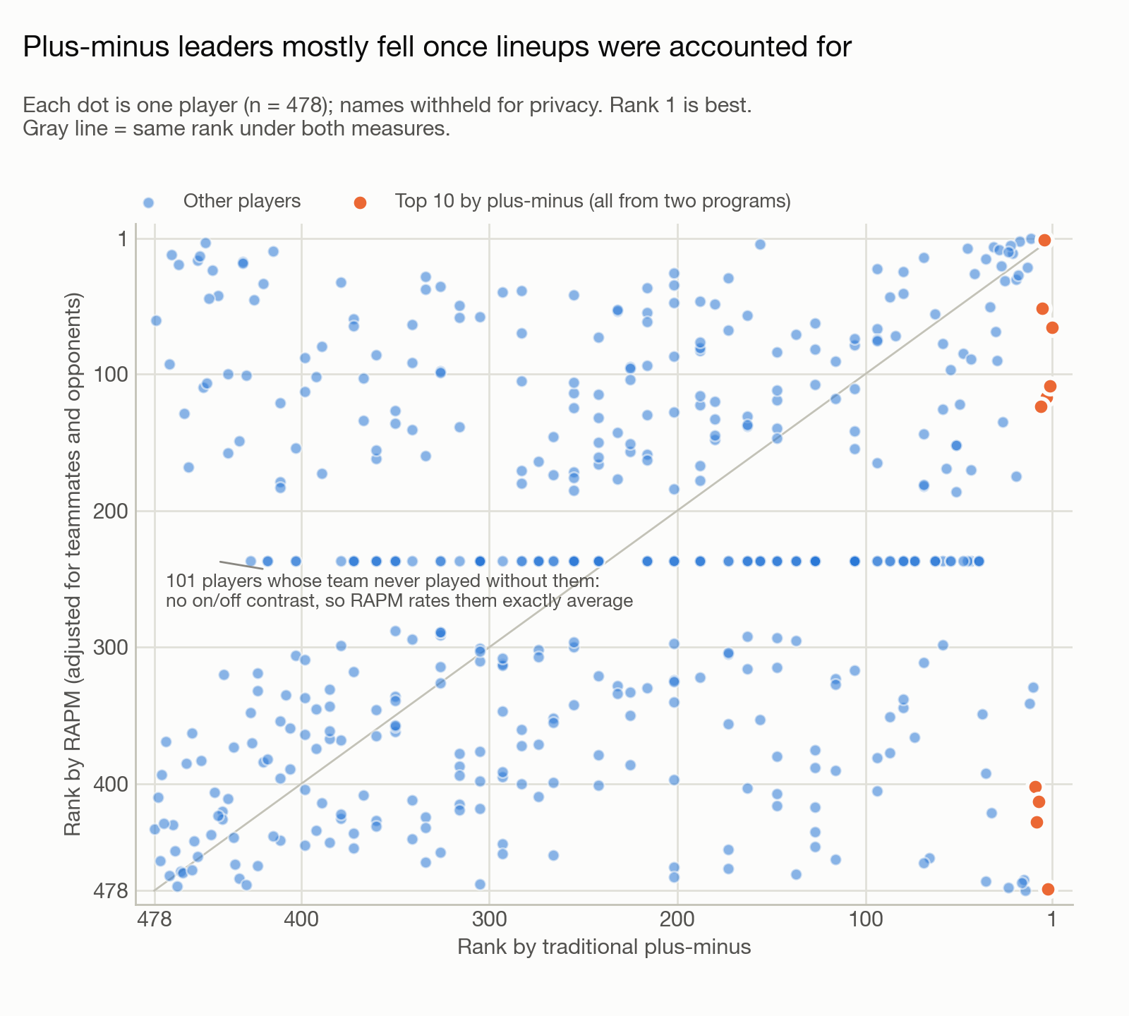
This was the type of adjustment the model was designed to make.

But it raised a more important question:

Were these new rankings actually reliable?

Testing rating stability

To test this, I randomly divided the season's matches into two halves.

I independently calculated player ratings using each half, then compared the resulting rankings using rank correlation.

The results revealed substantial differences in stability.

Rating method	Split-half rank correlation (approx.)
Production	0.75
Touch-level rating	0.55
Original RAPM	0.20
RAPM with stronger regularization	0.40–0.67

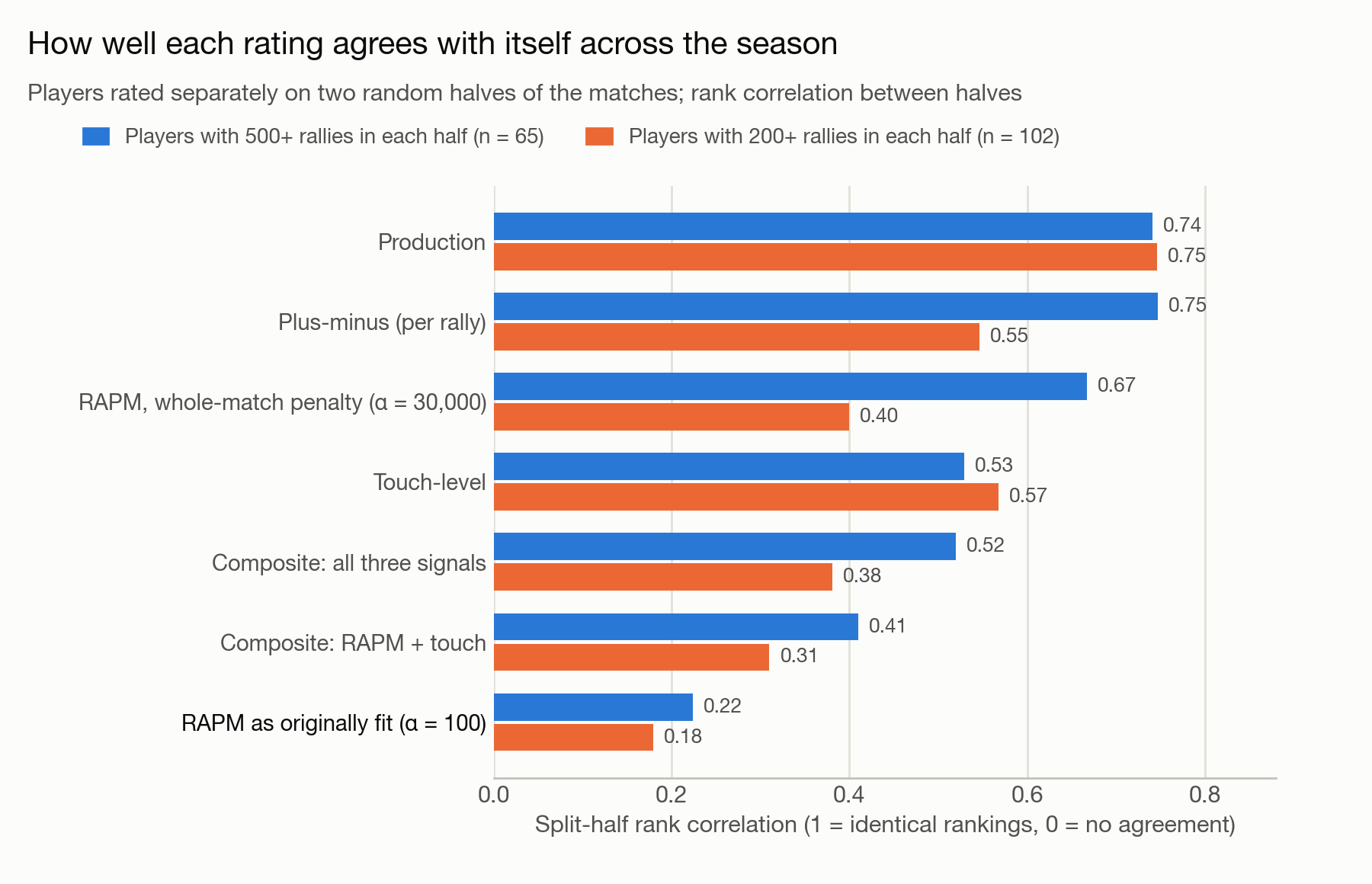
The original RAPM model (with a lambda of 100) showed relatively poor agreement between the two halves.

This suggested that its player ratings were highly sensitive to which matches were included.

After improving the validation strategy and increasing regularization, RAPM became considerably more stable.

However, it also became much more similar to traditional plus-minus.

This suggested that one season of data may not provide sufficient lineup variation to estimate individual effects reliably beyond broader team-level patterns.

Did combining the models actually help?

To evaluate the final ratings, I held out 45 matches.

I constructed the ratings using only the remaining matches, then tested whether they improved predictions of rally outcomes in the held-out matches.

The results were sobering.

None of the player-rating approaches, including the composite, outperformed a baseline that simply identified which two teams were playing.

Combining the signals improved the stability of the original RAPM-based ratings, but the composite remained less stable than the touch-level rating alone.

Therefore, I could not conclude that the composite was more accurate than its individual components.

Although the combined model was designed to capture complementary information, the available evidence did not demonstrate a predictive improvement.

What I would do differently

This project taught me as much about the limitations of statistical modeling as it did about implementing machine learning algorithms.

If I were to rebuild the system, I would make several changes.

1. Validate using entire matches from the beginning. Cross-validation must respect the structure of the data, especially when observations within a match are highly related.
2. Redesign the touch-level attribution method. Rather than predicting rally outcomes from events that may already reveal those outcomes, I would investigate a more direct estimate of the value associated with each graded touch.
3. Reconsider how the two models interact. Instead of simply averaging their outputs, I would explore using touch-based estimates as a starting point that RAPM adjusts. Players with substantial lineup variation could receive greater influence from RAPM, while players with limited lineup information could rely more heavily on touch-level evidence.
4. Pool multiple seasons of data to improve the reliability of individual player estimates.

Final thoughts

The goal of this project was to move beyond traditional volleyball statistics and investigate whether machine learning could provide a more complete understanding of individual player contributions.

RAPM offered a way to account for teammates, opponents, and game context.

Ridge regularization helped stabilize estimates in the presence of multicollinearity and limited data.

Touch-level modeling introduced information about the actions players actually performed.

However, combining these approaches did not automatically produce a better rating.

The most important lesson was that model complexity does not guarantee better measurement.

A model can be mathematically sophisticated, produce interesting rankings, and achieve strong predictive metrics while still failing to isolate the quantity we actually care about.

Ultimately, this project reinforced a broader principle of applied machine learning:

A model is only as meaningful as the assumptions behind it, the information available to it, and the evidence supporting its conclusions.

My goal was not to discover a perfect measure of volleyball talent, but to build, test, and critically evaluate a more context-aware approach to estimating individual contribution.